18. Biology – phylogeny

18.1. Motivation, prerequisites, plan

18.1.1. Motivation

One of the most important areas of research in biology is that of phylogenetic analysis. This collection of techniques allows us to build an evolutionary tree showing how various species are related.

This type of analysis can also be used in other areas, such as tracing the origin of human spoken languages.

I find phylogenetic analysis to be fascinating because it gives us a sort of “webcam of the gods”, a view of the past (which we cannot see) which brought about the present state of things.

18.1.2. Prerequisites

• The 10-hour “serious programming” course.

• The “Data files and first plots” mini-course in Starting out - data files and first plots

• Having the required libraries installed. Install them with:

$ sudo apt install python3-biopython python3-matplotlib

18.1.3. Plan

We will start by looking at a video tutorial of how to build a simple phylogenetic tree by hand. Then we will learn how to the biopython package to construct and visualize trees on that simple problem.

Then we discuss further projects in which we look for data sets to work with, including sets from our own genetic algorithm runs (where we also know the real evolutionary history), human languages (where we do not know the real history), and computer programming languages (where we should know most of the real history).

A book which summarizes the subject of taxonomy and phylogeny is here:

https://cnx.org/contents/24nI-KJ8@24.18:EmlvXoDL@7/Taxonomy-and-phylogeny

18.2. Start with a video and then make a simple table

Start with this Khan Academy tutorial on phylogenetic trees

Then we take their table of traits. Start with the empty table:

An empty trait table which the class could fill together.

Species	Feathers	Fur	Lungs	Gizzard	Jaws
Lamprey
Antelope
Sea Bass
Bald Eagle
Alligator

and write it on the board. Then fill out the tree on the board with the class. You can discuss what all these animals are, and look them up if necessary.

The table will end up looking like this:

What the trait table should like like once it is filled.

Species	Feathers	Fur	Lungs	Gizzard	Jaws
Lamprey	no	no	no	no	no
Antelope	no	yes	yes	no	yes
Sea Bass	no	no	no	no	yes
Bald Eagle	yes	no	yes	yes	yes
Alligator	no	no	yes	yes	yes

Then use the principle of parsimony to create the phylogenetic tree, following the guidelines in the tutorial. The result should look like what you see in Figure 18.2.1.

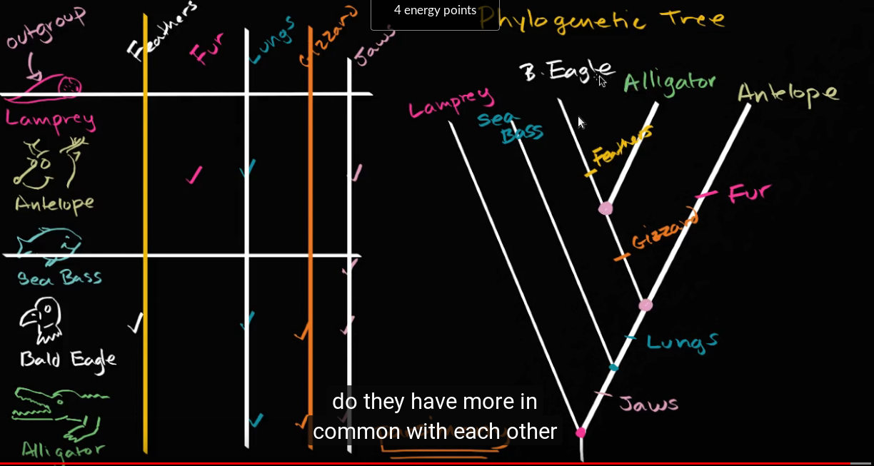
The resulting tree from the Khan Academy video example.

Discuss the meaning of parsimony as seen in this example. Connect it to Ockham’s razor.

Next we can look at Taylor Lindsay’s animal tree:

https://github.com/taylor-lindsay/phylogenetics/blob/master/images/animal_tree.png

and discuss how each branching-off involves the development of a new trait.

18.3. Terminology

Clades, taxa, species, genotype, phenotype, …

The tree of life

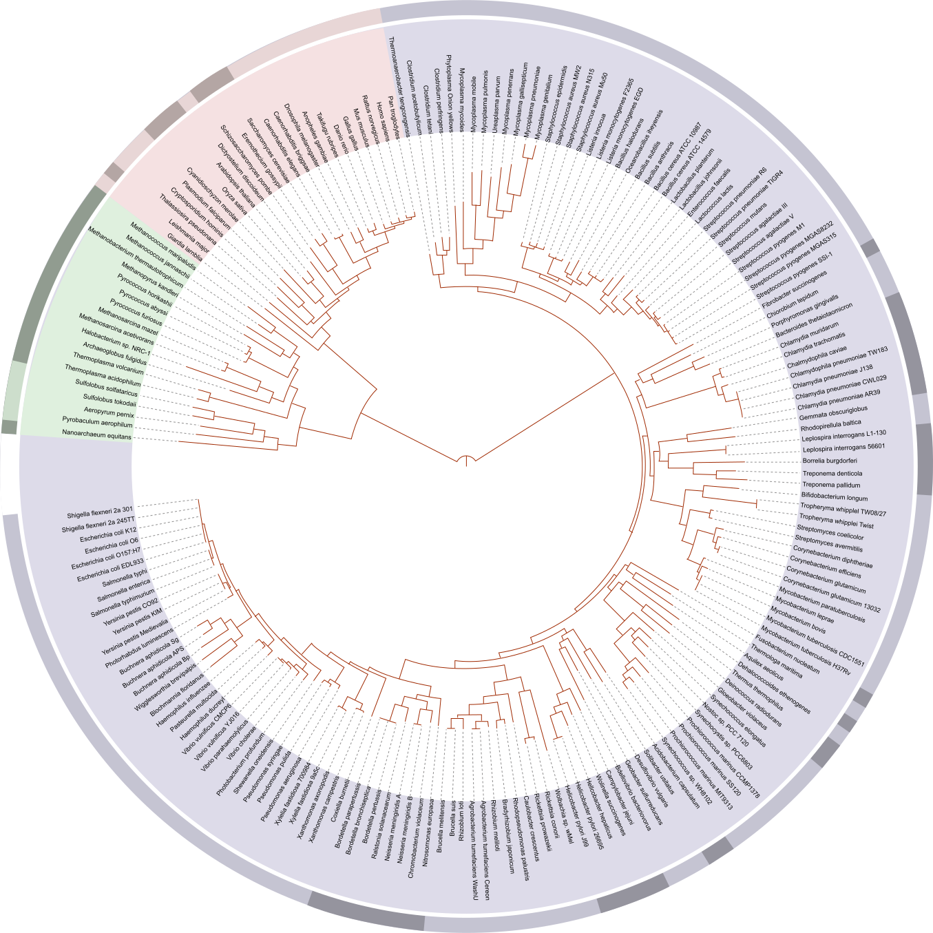
Figure 18.6.1 Hillis’s tree of life based on completely sequenced genomes (from the Wikipedia image)

There is an interactive tree of life here:

https://itol.embl.de/

18.4. First steps with biopython

Tutorials are at:

https://taylor-lindsay.github.io/phylogenetics/

and

http://biopython.org/DIST/docs/tutorial/Tutorial.html

The basic format of the library (or the part we will be using; biopython is HUGE) is below. You make a tree from some sort of text-based files (in this case just a string with some letters and parenthesis), then draw the tree. There are a lot of variations on this, but this is the fundemental structure.

from io import StringIO
from Bio import Phylo
from Bio.Phylo.TreeConstruction import DistanceCalculator
t = Phylo.read(StringIO("((a,b),c);" ), format="newick")
Phylo.draw(t)

18.5. Downloading the datasets

Data from opentreeoflife at:

https://tree.opentreeoflife.org/

I tied Streptococcus_mitis_NCTC_12261_ott725 at:

https://tree.opentreeoflife.org/opentree/argus/ottol@175918/Streptococcus

and downloaded the Newick format of the streptococcus subtree here.

with:

$ wget --output-document subtree-ottol-175918-Streptococcus.tre https://tree.opentreeoflife.org/opentree/default/download_subtree/ottol-id/175918/Streptococcus

And downloaded the opentreeoflife data with:

$ wget https://api.opentreeoflife.org/v3/study/ot_2221.tre

You can quickly visualize these datasets with:

import os
import matplotlib
import matplotlib.pyplot as plt
from Bio import Phylo
from Bio.Phylo.TreeConstruction import DistanceCalculator

tree = Phylo.read("ot_2221.tre", "newick")
Phylo.draw(tree)

tree = Phylo.read("subtree-ottol-175918-Streptococcus.tre", "newick")
Phylo.draw(tree)

Both are somewhat interesting to look ar

18.6. Preparing a tree by hand

Now let us prepare a tree where we input it ourselves. The format is like what we saw in the example above: the tree is made with the call Tree( "((a,b),c);" )

But we will make a slightly more interesting tree, the one we worked out in section Start with a video and then make a simple table. To do so enter the program in Listing 18.6.1.

Listing 18.7.1 Program which makes a phylogenetic tree from a simple example tree.

#! /usr/bin/env python3
import matplotlib.pyplot as plt
from io import StringIO
from Bio import Phylo
from Bio.Phylo.TreeConstruction import DistanceCalculator

t = Phylo.read(StringIO("((((Eagle,Alligator),Antelope),Sea Bass),Lamprey);" ), format="newick")
Phylo.draw(t)
Phylo.draw(t, do_show=False)
plt.savefig('simple-tree.png')
print('Saved tree to simple-tree.png')

You can adjust the look of this tree. See the discussion in the second tutorial link in the first steps section. We can go through that and adjust our styles a bit and see how our tree looks. That being said, here is what the above program should output:

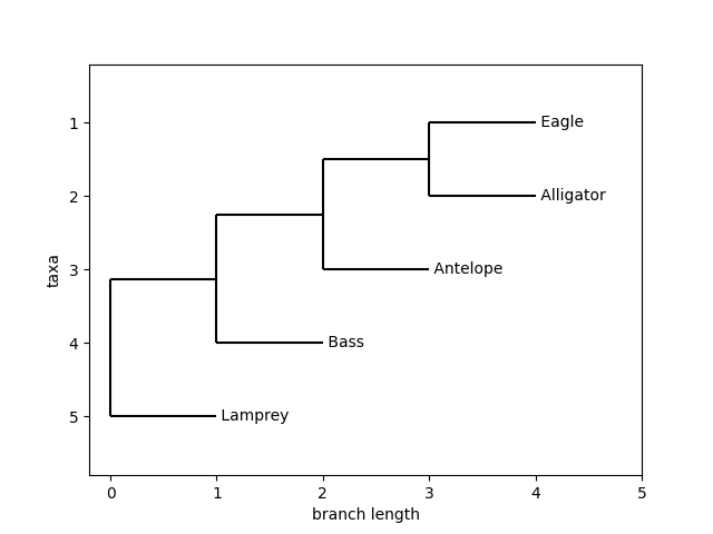
A version of the simple tree we deduced earlier.

18.7. Inferring a tree

The problem with the program in Listing 18.6.1 is that it visualizes the tree we created by hand. This is nice because you can view it with your favorite PNG or SVG file viewer. But it does not find the tree. That is our next goal.

So we want to find the most likely evolutionary tree that would yield the result we see in the Table 18.2.2. This process is called inferring the phylogenetic tree from the table of characteristics.

To do this, we will use the .fa (or fasta) file format to encode the information about traits. The format is fairly simple, with two lines per animal: one with an arrow and the name, like >lamprey, and then one with a single uppercase letter for each trait, like NNNNN. When we put all five animals into a file together, it will look something like:

simple-animals.fa - Table of traits for the animals we discussed earlier in Table 18.2.2

>Lamprey
NNNNN
>Antelope
NYYNY
>Sea_Bass
NNNNY
>Bald_Eagle
YNYYY
>Alligator
NNYYY

along with a program to infer a tree from it:

infer_tree.py - A simple program for inferring trees.

#! /usr/bin/env python3

import sys
import matplotlib.pyplot as plt

from Bio import Phylo
from Bio import AlignIO
from Bio.Phylo.TreeConstruction import DistanceTreeConstructor
from Bio.Phylo.TreeConstruction import DistanceCalculator

def main():
    fname = 'simple-animals.fa'
    if len(sys.argv) > 1:
        fname = sys.argv[1]
    file_format = 'fasta'
    if fname.endswith('.gb') or fname.endswith('.gbk'):
        file_format = 'genbank'
    print(fname, file_format)
    tree_alignment = AlignIO.read(fname, file_format)
    calculator = DistanceCalculator('identity')
    distance_matrix = calculator.get_distance(tree_alignment)
    constructor = DistanceTreeConstructor(calculator, 'upgma')
    tree = constructor.upgma(distance_matrix)
    Phylo.draw(tree)
    tree.root_with_outgroup('Lamprey') # maybe not?
    Phylo.draw(tree, do_show=False)
    plt.savefig('inferred_tree.png')
    Phylo.draw_ascii(tree)

main()

The output shows the same family links that we obtained by hand, but the tree looks different because the root is placed differently. To fix this, add tree.root_with_outgroup('Lamprey') directly before the final line. The reason this works is it gives the computer a sense of where to start, and creates the connections from there. If we hadn’t included it, as you can see in the figure below, it would have started from the point after the bass split off, giving a skewed view of the tree.

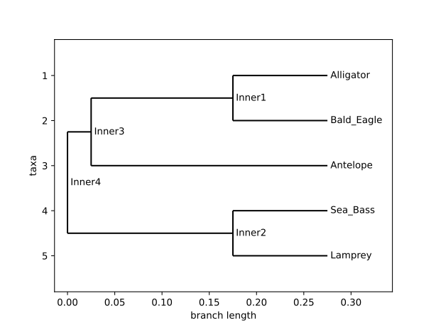
A tree with all the same connections, but the wrong root.

After applying the fix, the tree should look like this:

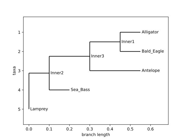
Figure 18.7.3 The correctly inferred tree.

You can also view this tree as ascii by replacing the Phylo.draw(tree) with Phylo.draw_ascii(tree).

We can save it to a file by adding a couple more lines:

import matplotlib.pyplot as plt
...

...
tree.root_with_outgroup('Lamprey')
Phylo.draw(tree, do_show=False)
plt.savefig('inferred_tree.png')
Phylo.draw_ascii(tree)

This will save a png formatted view of the tree, as well as showing you an ascii representation.

18.8. Inferring trees from real genetic data

Caution

From here on, at this time (2026-08-20), we are still forming a coherent set of examples. The links you will find below will be to various DNA sequences, but they are not yet all tested and clear.

The procedure gets much more elaborate. We will go in increasing steps. first we need to get a the mafft program to realign sequences so they can be compared:

sudo apt instal mafft

The sequence of steps for these “real world” examples, in our first rather simple application, will be:

18.8.1. The Biopython library example - lsorchid.fasta

More information on some of these examples

The national library of medicine (hosted by the National Institutes of Health, NIH) also stores the publications that went along with the sequencing of certain species. It is interesting, for exampole, to look at the paper that accompanies the California flannelbush (Fremontodendron californicum):

https://pmc.ncbi.nlm.nih.gov/articles/PMC13147169/

which has a link to downlolad the PDF of the paper.

One place to start with more realistic examples is from the biopython-provided example of several orchid species sequences. The example in the biopython documentation is here:

https://biopython.org/docs/latest/Tutorial/chapter_seqio.html

and the file ls_orchid.fasta is here:

https://raw.githubusercontent.com/biopython/biopython/refs/heads/master/Doc/examples/ls_orchid.fasta

and you can download the file with:

$ wget https://raw.githubusercontent.com/biopython/biopython/refs/heads/master/Doc/examples/ls_orchid.fasta

Then you can realign with:

$ mafft --auto ls_orchid.fasta > ls_orchid_realigned.fasta

You should now examine these two files visually to see:

ls_orchid.fasta

The original file had some 740 to 941 nucleotides in its sequences. Each sequence could have a different length.

ls_orchid_realigned.fasta

Each sequence now has the same length. Various sub-sequences of nucleotides have been moved around, and in some places sequences of dashes ------ have been inserted. This allows us to compare “apples to apples” in a certain sense: the gene subsequences that exist that don’t exist in a certain spcies are marked as ------ and not compared in calculating genetic differences.

18.8.2. The plague: Y.pestis

Or try Y.pestis from genbank. Check this page: https://www.ncbi.nlm.nih.gov/nuccore/NC_005816.1 and download with:

$ wget --output-file Y.pestis.gb 'https://www.ncbi.nlm.nih.gov/sviewer/viewer.cgi?tool=portal&save=file&log$=seqview&db=nuccore&report=genbank&id=45478711&&ncbi_phid=CE89312FA824C6B1000000000091008E'

or from reddit https://www.reddit.com/r/bioinformatics/comments/5h4qnc/what_is_the_best_way_to_download_genbank_data/

Saccharomyces cerevisiae
https://en.wikipedia.org/wiki/Accession_number_(bioinformatics)
locus=CP011547
curl -s  "https://eutils.ncbi.nlm.nih.gov/entrez/eutils/efetch.fcgi?db=nucleotide&id=${locus}&rettype=gb&retmode=txt" > ${locus}.gbk

for great whale shark:

locus=JAHMAH000000000

for Y.pestis: locus=CP160598.1

https://www.ncbi.nlm.nih.gov/datasets/taxonomy/7801/

https://www.ncbi.nlm.nih.gov/datasets/genome/?taxon=259920

Note

If our files are in genbank format then mafft (the alignment program) does not work onm that natively. You can convert a collection of .gbk files to a .fasta file with:

sudo apt install emboss any2fasta
for gbk_fname in *.gbk
do
    any2gbk $gbk_fname > ${gbk_fname}.fasta
done

Look at the .fasta files - they have very different sequence lengths, since you have sharks and orchids and plague bacteria. You can use mafft to realign them:

cat *.gbk.fasta > multi_species.fasta mafft –auto multi_species.fasta > multi_species_realigned.fasta

Now that we have a basic example out of the way, we are going to try a real-world example. This example is on variations a gene called CRAB across species, and can be copy-and-pasted from this link.

a larger fasta format file.

>crab_anapl ALPHA CRYSTALLIN B CHAIN (ALPHA(B)-CRYSTALLIN).             
MDITIHNPLIRRPLFSWLAPSRIFDQIFGEHLQESELLPASPSLSPFLMR
SPIFRMPSWLETGLSEMRLEKDKFSVNLDVKHFSPEELKVKVLGDMVEIH
GKHEERQDEHGFIAREFNRKYRIPADVDPLTITSSLSLDGVLTVSAPRKQ
SDVPERSIPITREEKPAIAGAQRK
>crab_bovin ALPHA CRYSTALLIN B CHAIN (ALPHA(B)-CRYSTALLIN).             
MDIAIHHPWIRRPFFPFHSPSRLFDQFFGEHLLESDLFPASTSLSPFYLR
PPSFLRAPSWIDTGLSEMRLEKDRFSVNLDVKHFSPEELKVKVLGDVIEV
HGKHEERQDEHGFISREFHRKYRIPADVDPLAITSSLSSDGVLTVNGPRK
QASGPERTIPITREEKPAVTAAPKK
>crab_chick ALPHA CRYSTALLIN B CHAIN (ALPHA(B)-CRYSTALLIN).             
MDITIHNPLVRRPLFSWLTPSRIFDQIFGEHLQESELLPTSPSLSPFLMR
SPFFRMPSWLETGLSEMRLEKDKFSVNLDVKHFSPEELKVKVLGDMIEIH
GKHEERQDEHGFIAREFSRKYRIPADVDPLTITSSLSLDGVLTVSAPRKQ
SDVPERSIPITREEKPAIAGSQRK
>crab_human ALPHA CRYSTALLIN B CHAIN (ALPHA(B)-CRYSTALLIN).
MDIAIHHPWIRRPFFPFHSPSRLFDQFFGEHLLESDLFPTSTSLSPFYLR
PPSFLRAPSWFDTGLSEMRLEKDRFSVNLDVKHFSPEELKVKVLGDVIEV
HGKHEERQDEHGFISREFHRKYRIPADVDPLTITSSLSSDGVLTVNGPRK
QVSGPERTIPITREEKPAVTAAPKK
>crab_mesau ALPHA CRYSTALLIN B CHAIN (ALPHA(B)-CRYSTALLIN).             
MDIAIHHPWIRRPFFPFHSPSRLFDQFFGEHLLESDLFSTATSLSPFYLR
PPSFLRAPSWIDTGLSEMRMEKDRFSVNLDVKHFSPEELKVKVLGDVVEV
HGKHEERQDEHGFISREFHRKYRIPADVDPLTITSSLSSDGVLTVNGPRK
QASGPERTIPITREEKPAVTAAPKK
>crab_mouse ALPHA CRYSTALLIN B CHAIN (ALPHA(B)-CRYSTALLIN) (P23).       
MDIAIHHPWIRRPFFPFHSPSRLFDQFFGEHLLESDLFSTATSLSPFYLR
PPSFLRAPSWIDTGLSEMRLEKDRFSVNLDVKHFSPEELKVKVLGDVIEV
HGKHEERQDEHGFISREFHRKYRIPADVDPLAITSSLSSDGVLTVNGPRK
QVSGPERTIPITREEKPAVAAAPKK
>crab_rabit ALPHA CRYSTALLIN B CHAIN (ALPHA(B)-CRYSTALLIN).             
MDIAIHHPWIRRPFFPFHSPSRLFDQFFGEHLLESDLFPTSTSLSPFYLR
PPSFLRAPSWIDTGLSEMRLEKDRFSVNLDVKHFSPEELKVKVLGDVIEV
HGKHEERQDEHGFISREFHRKYRIPADVDPLTITSSLSSDGVLTVNGPRK
QAPGPERTIPITREEKPAVTAAPKK
>crab_rat ALPHA CRYSTALLIN B CHAIN (ALPHA(B)-CRYSTALLIN).             
MDIAIHHPWIRRPFFPFHSPSRLFDQFFGEHLLESDLFSTATSLSPFYLR
PPSFLRAPSWIDTGLSEMRMEKDRFSVNLDVKHFSPEELKVKVLGDVIEV
HGKHEERQDEHGFISREFHRKYRIPADVDPLTITSSLSSDGVLTVNGPRK
QASGPERTIPITREEKPAVTAAPKK
>crab_squac ALPHA CRYSTALLIN B CHAIN (ALPHA(B)-CRYSTALLIN).             
MDIAIQHPWLRRPLFPSSIFPSRIFDQNFGEHFDPDLFPSFSSMLSPFYW
RMGAPMARMPSWAQTGLSELRLDKDKFAIHLDVKHFTPEELRVKILGDFI
EVQAQHEERQDEHGYVSREFHRKYKVPAGVDPLVITCSLSADGVLTITGP
RKVADVPERSVPISRDEKPAVAGPQQK

Note that you may have to trim the ends of the sequences to match the length; while this may lose some information contained in the sequences, it is small enough where the overall pattern will still show in the plot. We can reuse our tree-inferring program from earlier (make sure to change the file to the CRAB one and remove the line that sets the root), and it should produce something like Figure 18.7.3:

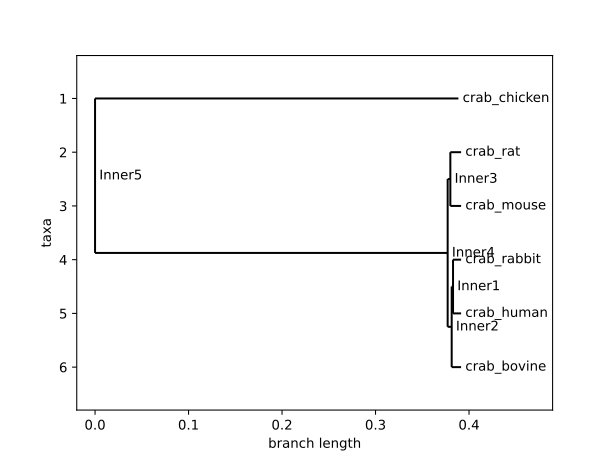
A graph showing the differences in the CRAB gene.

This graph shows a trend that makes a lot of sense: the mammals are all closely related, and the chicken is not closely related to them. In addition, the rat and mouse are closely related, which makes sense. The human in most closely related to the rabbit, and then the cow.

Biopython allowed us to learn all that information from meaningless (to us) sequences of letters. This can be incredibly useful for building phylogenetic trees, because you can simply plug in the genomes you are comparing and it will tell you how they are related. It’s not perfect, as we saw, and you may have to define an outgroup to “orient” the program. But other than that, it worked very well, and could build both or specifically engineered tree and a real example of a genome.

This is only a small taste of what biopython can do, and exploring it further would be reqrding for those with an interest in biology. The documentation and examples can be found here.

18.9. Other sequence analysis resources

Berkeley evolution course. 7 organisms and 7 features: https://evolution.berkeley.edu/evolibrary/article/phylogenetics_07

Cute with ladybugs, but just 6 elements and 7 features: https://bioenv.gu.se/digitalAssets/1580/1580956_fyltreeeng.pdf

Another video giving step-by-step for building a tree by hand: https://www.youtube.com/watch?v=09eD4A_HxVQ

18.10. Linguistics datasets

First discuss the issues of generating a string representation of language features. One example of the issues involved is given in this article:

https://brill.com/view/journals/ldc/3/2/article-p245_4.xml?lang=en

where they discuss how to align the English “horn” with the latin “kornu”. This then allows you to define a “genetic distance” between the same word in two different languages. One such measure is the “Levenshtein normalized distance” (LDN), which takes values between 0 and 1.

This can then be used with the ASJP (Automated Similarity Judgement Program) https://en.wikipedia.org/wiki/Automated_Similarity_Judgment_Program database which is based on a word list. The database is at https://asjp.clld.org/

Download the database from

https://asjp.clld.org/download

and look at the listss18.txt file and see how languages we know (English, Italian, Spanish, Russian) are represented.

Look at the results in WorldLanguageTree001.pdf

One oft-used list is the the Swadesh list https://en.wikipedia.org/wiki/Swadesh_list which has 100 terms. Some of these are “I”, “you”, “we”, “this”, “that”, “person”, “fish”, “dog”, “foot”, “hand”, “sun”, “mountain”, various basic colors, and so forth. There is also an abbreviated 35-word list. The ASJP uses a 40-word list, similar to the Swadesh list.

Each part of a word gets an ASJP code and an IPA (International Phonetic Alphabet) designation of how it’s pronounced.

18.10.1. lingpy.org

Go through the tutorial, starting at:

http://www.lingpy.org/tutorial/index.html

install with

pip3 install lingpy

then simple examples at:

http://www.lingpy.org/examples.html

then the workflow tutorial at:

http://www.lingpy.org/tutorial/workflow.html

and the cookbook at:

https://github.com/lingpy/cookbook

18.10.2. elinguistics.com

Overall language evolutionary tree: http://www.elinguistics.net/Language_Evolutionary_Tree.html You can follow the links to some detailed discussion of timelines at http://www.elinguistics.net/Language_Timelines.html as well as in-depth discussion of encoding and language comparison. In particular you will find various sounds for key encoding words at http://www.elinguistics.net/Compare_Languages.aspx?Language1=English&Language2=German&Order=Details

The choice of “basis words” to use as “genetic markers” is described at http://www.elinguistics.net/Lexical_comparison.html and the continuing pages http://www.elinguistics.net/Sound_Correspondence.html and back to the example of English to German at http://www.elinguistics.net/Compare_Languages.aspx?Language1=English&Language2=German&Order=Details

18.10.3. Others

https://en.wikipedia.org/wiki/Tree_model#Perfect_phylogenies

https://en.wikipedia.org/wiki/Tree_model

https://en.wikipedia.org/wiki/Language_family

https://en.wikipedia.org/wiki/Tree_model#CITEREFNakhleh2005

https://www.theguardian.com/education/gallery/2015/jan/23/a-language-family-tree-in-pictures

https://www.ncbi.nlm.nih.gov/pmc/articles/PMC3049109/

https://linguistics.stackexchange.com/questions/14905/is-there-a-phylogenetic-tree-for-all-known-languages

https://glottolog.org/

https://glottolog.org/resource/languoid/id/stan1293

https://glottolog.org/glottolog/family

https://www.ethnologue.com/browse/families

https://glottolog.org/resource/languoid/id/macr1271

https://science.sciencemag.org/content/323/5913/479

Look at the PDF for this paper on phylogeny of polynesian languages:

https://www.researchgate.net/publication/23933879_Language_Phylogenies_Reveal_Expansion_Pulses_and_Pauses_in_Pacific_Settlement

And this one with very nice-looking pictures of Japonic language evolution and some discussion of word differentiation.

https://royalsocietypublishing.org/doi/full/10.1098/rspb.2011.0518

Natural language processing with Python and NLTK:

http://www.nltk.org/book/

18.11. Evolution of programming languages

https://www.i-programmer.info/news/98-languages/8809-the-evolution-of-programming-languages.html

https://royalsocietypublishing.org/doi/full/10.1098/rsif.2015.0249